Mastering Apache Spark Partitioning: Coalesce vs. Repartition

Optimizing Performance Through Strategic Data Distribution

In the world of big data processing, understanding how your data is distributed across a cluster is crucial for performance optimization. Apache Spark, one of the most popular distributed computing frameworks, offers two primary methods for controlling data partitioning: coalesce() and repartition().

While these functions might seem similar at first glance, their differences can dramatically impact your Spark job's performance, resource utilization, and execution time.

Understanding Partitions in Apache Spark

Before diving into the specifics of coalesce and repartition, let's clarify what partitions are in Spark. A partition is simply a chunk of your dataset that can be processed by a single executor thread. The number of partitions determines the level of parallelism in your Spark job - more partitions generally mean more tasks running concurrently.

When you load data into Spark or perform transformations like join() or groupBy(), Spark automatically determines the number of partitions. However, there are many scenarios where you might want to manually control this partitioning, which is where coalesce() and repartition() come into play.

Coalesce: The Narrow Transformation

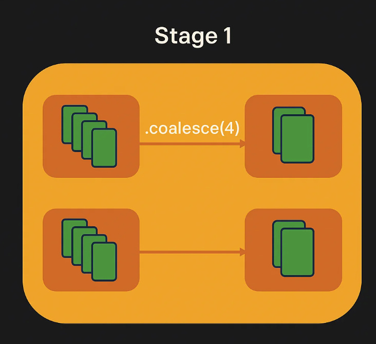
coalesce(n) is designed to reduce the number of partitions in your DataFrame without triggering a full data shuffle. It's considered a "narrow transformation" because it only combines existing partitions rather than redistributing data across the entire cluster, for example:

val reducedDF = originalDF.coalesce(4)

Will combine partitions in a given node, so no shuffle is triggered and we stay in the same stage:

Key characteristics of coalesce:

• One-way operation: Coalesce can only reduce the number of partitions, not increase them (unless you set shuffle=true, which essentially turns it into repartition).

• Minimal data movement: It attempts to combine partitions that are already on the same executor, minimizing network traffic.

• Potentially uneven distribution: The resulting partitions may have skewed sizes because data is not reshuffled.
  

Repartition: The Wide Transformation

repartition(n) both increases and decreases the number of partitions with a full shuffle, evenly redistributing the data across the cluster. It's a "wide transformation" because each output partition may depend on data from all input partitions. This will create 16 partitions that are evenly distributed and a new stage will be created:

val evenlyDistributedDF = originalDF.repartition(16)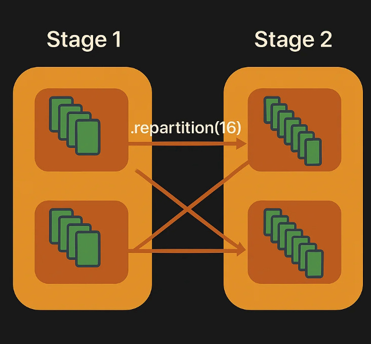

Key characteristics of repartition:

• Bidirectional operation: Can both increase and decrease the number of partitions.

• Full data shuffle: Triggers a complete redistribution of data across the cluster.

• Even distribution: Produces roughly equal-sized partitions, which is optimal for parallel processing.

• Under the hood: Technically, repartition(n) is implemented as coalesce(n, shuffle=true).

For a more in-depth read on wide and narrow transformations, check our post on this topic.

The Hidden Drawbacks: Performance Implications

While these operations seem straightforward, they come with significant performance implications that aren't immediately obvious.

The Shuffle Cost of Repartition

Repartition's full data shuffle is expensive:

• It requires all data to be serialized, transmitted across the network, and deserialized.

• This network transfer and serialization/deserialization adds significant overhead.

• The shuffle operation creates new stage boundaries in your Spark job.

Coalesce's Stage-Wide Impact

Coalesce has a less obvious but potentially more insidious impact:

• Stage-wide partition limitation: Coalesce is a narrow transformation that affects the entire stage it belongs to in Spark's execution plan.

• In Spark, a stage is a collection of tasks that can be executed without requiring a shuffle.

• When you add a coalesce(n) operation, all operations within that same stage will run with at most n tasks.

For example, imagine you have a cluster with 100 cores available for processing, and your data initially has 200 partitions. Each partition is processed by one core, so all 100 cores would be busy (running two waves of tasks) during processing.

But watch what happens when you add a coalesce operation to your pipeline:

val df = spark.read.parquet("/large-dataset")
val result = df.map(complexTransformation)
               .filter(expensiveCondition)
               .coalesce(10)
               .write.parquet("/output")

What should happen is that your map and filter operations would use all 100 cores fully. However, in reality, the entire pipeline is limited to only 10 tasks because of the coalesce operation.

This means 90 cores (90% of your cluster) sit completely idle during this job, and it takes approximately 10 times longer than it should have!

This emphasizes that even naive changes that should help, lead to devastating results.

It's not that Spark reorders your operations - it's that Spark's execution model organizes these narrow transformations into a single stage with the partition count limited by the coalesce.

Common Confusion: "Why Aren't My Partitions Changing?"

One frequent source of confusion is when users call coalesce() or repartition() and don't see an immediate effect. For example:

val df = spark.read.parquet("/data")
println(df.rdd.getNumPartitions) // Shows original count, e.g., 200

val newDF = df.coalesce(10)
println(newDF.rdd.getNumPartitions) // Still shows 200! What's happening?

This happens because of Spark's lazy evaluation model. Transformations like coalesce() and repartition() don't execute until an action is triggered. To see the effect, you need to:

// Force an action
newDF.count()
println(newDF.rdd.getNumPartitions) // Now shows 10

Or directly chain to an action:

df.coalesce(10).write.parquet("/output") // Will produce 10 files

3 Performance Tips for Partitioning in Spark

1. Avoid Reducing to Very Low Numbers (Both Coalesce and Repartition)

Be extremely cautious when reducing partitions to low numbers with either operation:

df.coalesce(1).write.parquet("/output-coalesce")
df.repartition(1).write.parquet("/output-repartition")

Remember that your entire dataset must fit into the number of partitions you specify, and if there's not enough RAM in your executor machines, this will lead to out-of-memory errors.

This memory concern applies equally to both coalesce and repartition operations. The difference is in how they get there (coalesce avoids a shuffle, repartition does a full shuffle), but the end result of having very few partitions creates the same memory pressure on executors.

This is especially problematic with reducing to a single partition when working with large datasets, as it forces the entire dataset to be processed by a single executor thread. Even though the data doesn't all move to the driver (a common misconception), it still needs to fit in a single executor's memory allocation.

For large datasets, maintain enough partitions to keep memory requirements per partition reasonable, how many? see the next tip.

2. Balance Partition Count with Data Size

Aim for partition sizes between 100MB and a few GB for optimal performance:

• Too few partitions: Underutilizes cluster resources and can cause memory issues

• Too many partitions: Creates overhead from task scheduling and tiny files

A helpful rule of thumb:

Target partitions ≈ (total data size / target partition size)

Where the target partition size is typically 128MB-512MB depending on your workload.

3. Use Repartition for Skewed Data

When your data distribution is highly skewed (e.g., after filtering out 99% of records or joining on a non-uniform key):

// After a heavy filter, data is likely skewed
val filteredDF = df.filter(heavyFilter) // Maybe only 1% of records remain

// Bad: Maintains skew, some partitions may be nearly empty
filteredDF.coalesce(20).write.parquet("/output")

// Good: Redistributes data evenly
filteredDF.repartition(20).write.parquet("/output")

The small overhead of a shuffle is often worth it to achieve balanced partitions for subsequent operations.

Why Understanding Partitioning Is Critical for Performance

Partitioning is one of the most fundamental aspects of Spark's distributed computing model. Getting it right can mean the difference between a job that completes in minutes versus hours, or between a job that succeeds versus one that fails with out-of-memory errors.

Proper partitioning allows you to:

1. Maximize resource utilization: Ensure all your cores are working efficiently without idle executors or stragglers.

2. Minimize network transfer: Reduce expensive shuffle operations when possible.

3. Optimize storage patterns: Control the number and size of output files.

4. Prevent memory issues: Avoid creating partitions too large for a single executor to handle.

In practice, many Spark jobs suffering from poor performance can be dramatically improved just by adjusting partitioning strategies. Whether it's avoiding an unnecessary shuffle with a well-placed coalesce, or breaking up a skewed dataset with a strategic repartition, understanding these operations is a crucial skill for any Spark developer.

Conclusion

The choice between coalesce and repartition isn't simply about "which is faster" - it's about understanding the trade-offs and applying the right tool at the right time. Coalesce avoids expensive shuffles but can lead to skewed partitions and potentially limit parallelism. Repartition ensures even distribution but at the cost of a full shuffle.

By understanding these nuances and following the best practices outlined above, you can significantly improve your Spark jobs' performance and make more efficient use of your cluster resources.