Understanding Wide vs. Narrow Transformations in Apache Spark: Why It Matters for Performance

Optimize Your Spark Jobs by Understanding Data Dependencies and Shuffle Operations

When working with Apache Spark for big data processing, understanding the difference between wide and narrow transformations is crucial for optimizing your data processing pipelines.

Following last week's post, "Transformations vs. Actions in Apache Spark: The Key to Efficient Data Processing," this article goes deeper and focuses specifically on wide vs. narrow transformations.

This distinction directly impacts how Spark executes your code, affects performance, and determines how data flows through your application. Let's dive into what these transformations are and why they matter for your Spark performance tuning.

What are Narrow and Wide Transformations in Spark?

Narrow Transformations

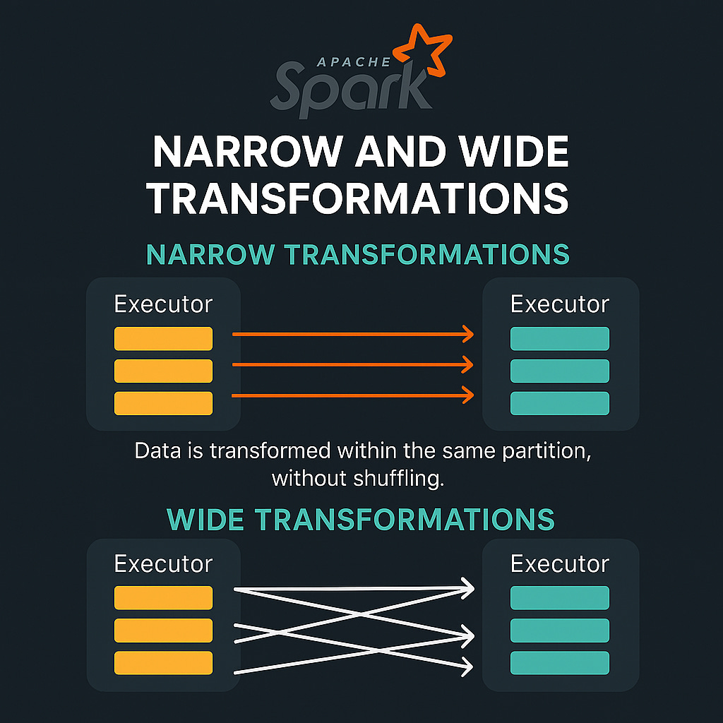
Narrow transformations are operations where each partition of the output DataFrame depends on at most one partition of the parent DataFrame. In simpler terms, the data required to compute an output record comes from only one input partition.

Key characteristics of narrow transformations:

• They don't require data from other partitions

• They can be executed independently on each partition

• Data doesn't need to be shuffled across the cluster

• Examples include: select(), selectExpr(), filter(), where(), withColumn(), drop(), union(), sample(), explode(), and load()

Wide Transformations

Wide transformations, on the other hand, are operations where each partition of the output may depend on data from multiple partitions of the input. This means data from different partitions needs to be combined.

Key characteristics of wide transformations:

• They require data from multiple partitions

• They involve data shuffling across the cluster

• They create stage boundaries in the execution plan

• Examples include: groupBy(), agg(), join(), orderBy(), sort(), distinct(), pivot(), and operations that use window functions

When Does Shuffling Occur?

A shuffle happens during wide transformations when Spark needs to redistribute data across partitions, typically when we need to bring together records with the same keys. For more info, check our previous post explaining shuffle in-depth.

For example:

• In a join() operation, records with matching keys need to be brought together

• During groupBy(), all values for the same key must be collected in one place

• With distinct(), duplicate records need to be eliminated, requiring comparison across partitions

Shuffling is an expensive operation because it involves:

• Disk I/O (writing shuffle files)

• Network I/O (transferring data between nodes)

• Serialization and deserialization of data

How Spark Stages Relate to Transformations

Apache Spark divides the execution of your job into stages, and these stages directly correspond to the shuffle boundaries created by wide transformations:

1. DAG (Directed Acyclic Graph): Spark first creates a logical execution plan represented as a DAG.

2. Stage Division: The DAG is divided into stages at shuffle boundaries (wide transformations).

3. Task Creation: Within each stage, Spark creates tasks that can execute in parallel across partitions.

A key insight: A sequence of narrow transformations can be executed together as a single stage, with the operations being "pipelined" for efficiency. However, each wide transformation typically forces a new stage to begin, as Spark needs to complete the shuffle before proceeding.

Common Confusions About Wide vs. Narrow Transformations

One frequent point of confusion is understanding why some operations that seem to combine or modify data don't cause shuffles. For example:

union() vs. intersection():

• union() is a narrow transformation because it simply combines partitions from two DataFrames without redistributing data. It's like stacking one dataset on top of another.

• intersection() is a wide transformation because Spark needs to compare elements across all partitions to find common ones, requiring a shuffle.

Another common misconception is thinking that operations that change key values (like withColumn or using an expression in select) will trigger shuffles. These transformations that change keys are still narrow because:

• The transformation itself happens locally within each partition

• No data needs to move between partitions during the map

• Only a subsequent wide operation (like a join or groupBy on the new keys) would trigger a shuffle

Performance Tips for Managing Spark Transformations

1. Minimize Shuffle Operations in Spark

Since wide transformations are expensive, try to reduce their number:

// Less efficient: Two shuffles (groupBy + join)
val grouped1 = data1.groupBy("key").agg(...)
val grouped2 = data2.groupBy("key").agg(...)
val result = grouped1.join(grouped2, "key")

// More efficient: One shuffle (join first, then aggregate)
val joined = data1.join(data2, "key")
val result = joined.groupBy("key").agg(...)

2. Optimize Partition Count for Shuffles

The default number of shuffle partitions (200) isn't optimal for all workloads.

Rule of thumb: aim for partitions 2-3x the number of cores

• For small datasets or local development, reduce this number to avoid overhead:

spark.conf.set("spark.sql.shuffle.partitions", 4) // For small local jobs

• For large production jobs, ensure enough partitions to distribute work evenly:

spark.conf.set("spark.sql.shuffle.partitions", 300) // For a 100-core cluster

3. Handle Data Skew in Wide Transformations

Data skew (when some keys have far more data than others) can severely impact shuffle performance:

• Since Spark 3.0 Adaptive Query Execution (AQE) was introduced to automatically rebalance skewed joins, check if its on.

• Consider techniques like salting keys to distribute hot keys across partitions

Why Understanding Spark Transformations Is Critical for Performance

The distinction between wide and narrow transformations fundamentally affects Spark's execution model and performance in several ways:

1. Resource Consumption: Wide transformations require more memory, disk space, and network bandwidth due to shuffling.

2. Execution Time: Jobs with many wide transformations will take longer to complete due to the overhead of shuffling data.

3. Failure Recovery: Narrow transformations allow for faster recovery since lost partitions can be recomputed independently, while wide transformations may require recomputing entire stages.

4. Optimization Opportunities: Understanding these patterns allows you to restructure your code to minimize shuffles and optimize performance.

By examining your Spark UI, you can identify stages and shuffles in your application. Look for:

• Stage boundaries, which indicate shuffle operations

• The amount of data being shuffled (Shuffle Read/Write metrics)

• Tasks that take significantly longer than others (potential data skew issues)

For additional performance insights, consider using tools like Dataflint open source to identify bottlenecks in your Spark jobs.

Conclusion: Mastering Spark Performance Through Transformation Knowledge

Mastering the concepts of wide vs. narrow transformations is fundamental to writing efficient Apache Spark applications. By minimizing wide transformations where possible, properly configuring shuffle partitions, and addressing data skew, you can significantly improve the performance of your Spark DataFrame operations.

Remember that every wide transformation introduces a synchronization point in your distributed computation, so they should be used judiciously. The next time you write a Spark application, consider how data flows through your transformations and look for opportunities to optimize shuffle operations for better Spark performance.

Have you optimized your Spark jobs by reducing shuffle operations? Share your experiences in the comments below!